Writing a Neural Network from Scratch in Rust

Published February 24, 2022

It’s what powers nearly all of modern artificial intelligence, from facial recognition to natural language processing: Neural Networks. Lying beneath the buzzwords and marketing jargon exists a powerful optimization machine which we will attempt to understand today.

High Level Explanation

While the mathematical notation and vocabulary surrounding Nerual Nets seems intimidating, the high level overview of what these machines do and how they learn can be quite tangible.

The first thing we need to define is our goal. What is the neural network supposed to do for us? Put simply, we feed it some data, it gives us some result. For instance, we could feed it a picture, and as a result we want to know whether the image is of a cat or a dog. Similarly, we could feed it movie reviews expecting to know whether the review was positive or negative.

For now let’s think of a neural network as a giant mess of math equations. What these equations are or how they work doesn’t matter right now, all we know is we pipe our data into the equation and we get an answer out. This process of sending the data through the neural network is referred to as “forward propogation”.

So we take some spare cat photos that we have lying around on our hard drives and start pumping them through the network. The results are completely inaccurate, many of your cats being mislabeled as dogs.

We know some of the results are wrong, but it is critical to know how wrong. We look at the total number of cat photos and count how many were incorrectly identified as dogs. This is what we call our “cost” or “loss”. It is how we measure the error in our neural network.

What happens next is the magic which makes the whole system work. Our mess of mathematical equations has a super power; while sending data through one side yields predictions, sending the error through the equations backwards modifies the internal structure of our math equations, and the network learns! This process of sending the error backwards through the network is aptly named “backpropagation”.

So we repeat this process many times with as many photos as we can gather. First sending the photos through and measuring our error and then sending our error backwards through the network, over and over again until we have a network that can properly label all of the internet’s cat photos.

Some more (but still probably not enough) details

Let’s get a little more specific about the internal structure of our neural network. You may have seen diagrams that look similar to the following:

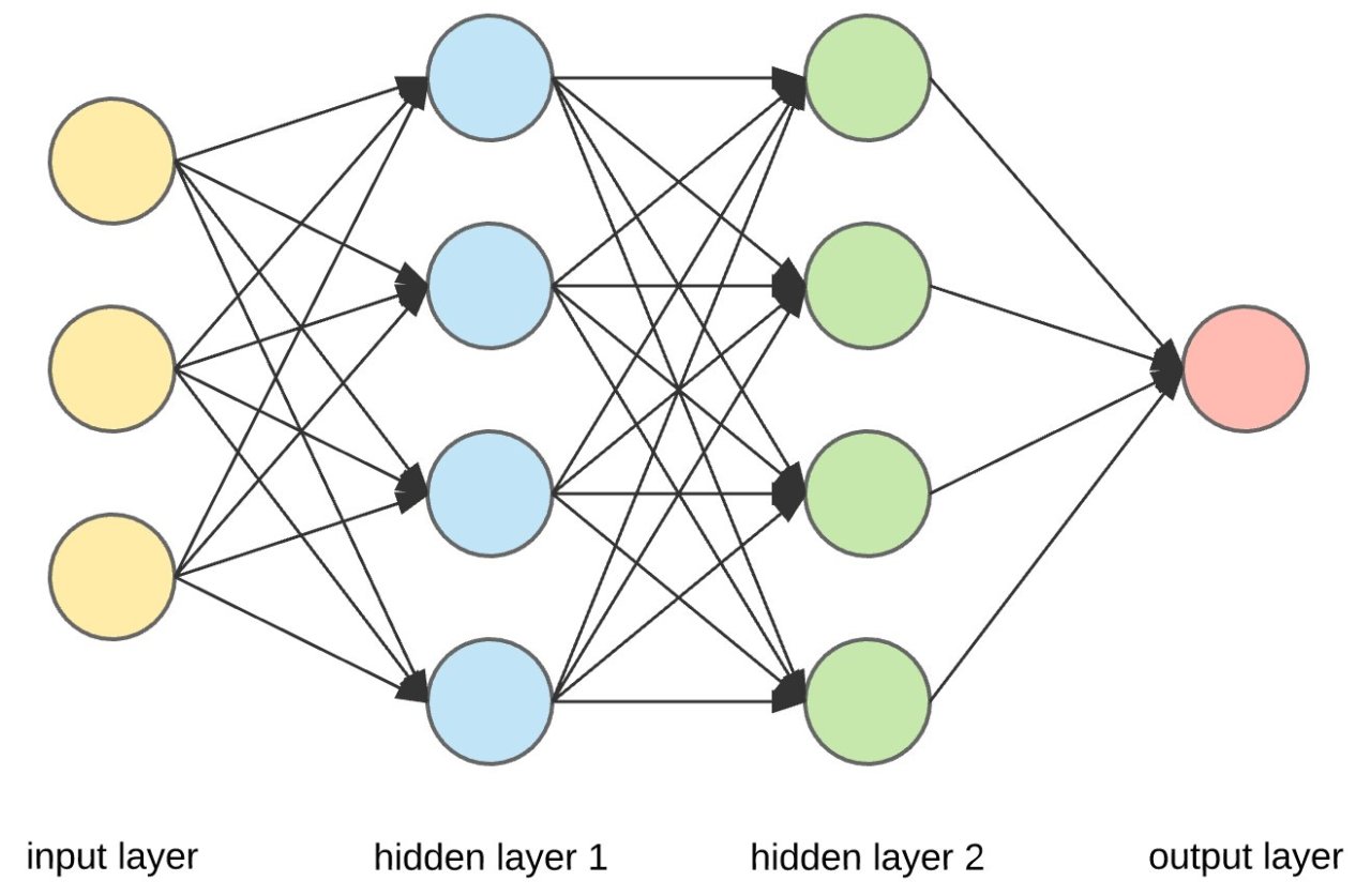
There’s quite a bit going on in that diagram, too much for now, so let’s focus on a much simpler network.

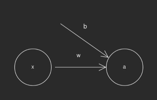
This simple network consists of a few basic elements: the input x, the weight w, the bias b, and the output a. The formula for our forward propogation, a as a function of x, is simply a = activation(w*x+b). activation in this case is a activation function which can denoise and add necessary non-linearites to our network. The right activation function can allow nodes to be turned off or normalized to more sane values. In most networks you will see relatively simple functions such as the sigmoid or ReLu.

What happens when we have multiple inputs?

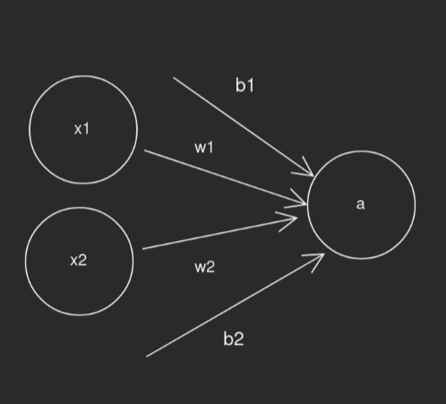
Our formula still remains rather simple, instead of a single linear equation we have a linear combination piped throught the activation function: a = activation(w1*x1+b1 + w2*x2+b2).

This is where linear algebra comes in to make our lives much easier. Since the bulk of the calculations for any network is represented by a series of linear combinations, we can easily represent our network through a series of matrix multiplications. Thus our inputs become an input vectore, multiplied by our weight matrix added with our bias vector. For each layer that we want to add inbetween we define another weight matrix and bias vector.

This makes representing complex networks such as the one pictured above trivial. Each layer amounts to a single matrix multiply, a vector add, and applying the activation function to each member of the output vector.

This is only half the equation, the forward propogation part of network. We have yet to understand how the backpropagation works. The process which gives our backpropagation its power is known as gradient descent, and it involves subtracting from each weight its derivative with respect to the error, or in essence how much that particular weight contributed to the error. For now this is where my explanation of gradient descent stops, as I have yet to cement my understanding of the math behind it and am still questioning the correctness of my matrix implementation. It is better that I admit my own shortcomings than if someone was to be misled by my flawed understanding.

Code

Rust, Const Generics, and Matrices

Let’s get to some code! For the matrix class I used the relatively new rust feature of const generics, which allows for compile time constants to be passed as part of a objects type signature. This allowed for some pretty neat things, like checking my matrix multiplications at compile time! A slimmed down version of my matrix struct is as follows:

/// Trait that defines necessary behaviour for matrix cell type
pub trait MatrixCell<T>: Default + Clone + Copy {} //+ other mathematical traits
impl MatrixCell<f32> for f32 {}

/// Actual Matrix Type
#[derive(Clone, Copy, Debug, PartialEq)]
pub struct Matrix<T, const HEIGHT: usize, const WIDTH: usize> {
    data: [[T; WIDTH]; HEIGHT]
}

/// Implement matrix multiplication (naive)
impl<T, const WIDTH: usize, const HEIGHT: usize, const OTHER_WIDTH: usize>
std::ops::Mul<Matrix<T, WIDTH, OTHER_WIDTH>> for Matrix<T, HEIGHT, WIDTH>
where T: MatrixCell<T> {
    type Output = Matrix<T, HEIGHT, OTHER_WIDTH>;

    fn mul(self, rhs: Matrix<T, WIDTH, OTHER_WIDTH>) -> Self::Output {
        let mut out = Matrix::<T, HEIGHT, OTHER_WIDTH>::new();

        for i in 0..HEIGHT {
            for j in 0..OTHER_WIDTH {
                let mut sum = T::default();

                for k in 0..WIDTH {
                    sum += self.data[i][k]*rhs.data[k][j];
                }

                out.data[i][j] = sum;
            }
        }

        out
    }
}

// More Implementations of other operators

This syntax is pretty dense and definitely took a while to get used to, but it provides a beautiful simple abstraction for working with matrices where we can check our operations at compile time. For instance, given the following code segment where we try to multiply two matrices with incompatible dimensions:

let m1 = Matrix::<f32, 5, 2>::new();
let m2 = Matrix::<f32, 3, 3>::new();
let m3 = m1 * m2;

The compiler would inform us that they have incompatible types!

Network Definition

For this example we will be using the MNIST dataset, a dataset full of images of handwritten characters. The goal will be to take an image of a handwritten digit and correctly classify it. We can set up the weights and biases for a network to handle the 784 input pixels with a few hidden layers as so:

let mut w1 = Matrix::<f32, 128, 784>::random();
let mut w2 = Matrix::<f32, 64, 128>::random();
let mut w3 = Matrix::<f32, 10, 64>::random();

let mut b1 = Matrix::<f32, 128, 1>::new();
let mut b2 = Matrix::<f32, 64, 1>::new();
let mut b3 = Matrix::<f32, 10, 1>::new();

Forward Propogation

Using our matrix multiplications, we work through each layer calculating the linear combination of the weights with the inputs and biases while passing everything through our activation function, sigmoid:

let z1 = w1*x + b1;
let a1 = z1.apply(sigmoid);
let z2 = w2*a1 + b2;
let a2 = z2.apply(sigmoid);
let z3 = w3*a2 + b3;
let a3 = z3.apply(sigmoid);

Backwards propogation

Using the difference between our prediction and the actual result, calculate the necessary change to each layer of weights and biases:

let diff = a3-*y;

let da3 = diff * 2.0;
let dz3 = a3.apply(sigmoid_d).hadamard(da3);
let dw3 = dz3 * a2.transpose();
let db3 = dz3;

let da2 = w3.transpose() * dz3;
let dz2 = a2.apply(sigmoid_d).hadamard(da2);
let dw2 = dz2 * a1.transpose();
let db2 = dz2;

let da1 = w2.transpose() * dz2;
let dz1 = a1.apply(sigmoid_d).hadamard(da1);
let dw1 = dz1 * x.transpose();
let db1 = dz1;

Apply the changes

Finally we can take these derivatives that we have calculated and subtract them from our current weights and biases (multiplied by a constant learning rate).

w3 -= dw3 * r;
w2 -= dw2 * r;
w1 -= dw1 * r;

b3 -= db3 * r;
b2 -= db2 * r;
b1 -= db1 * r;

Conclusion

There you have it, a mostly rushed half-baked implementation of a neural network in rust. The complete source code can be found on my github.

If you find any errors in this article or in my source code, feel free to reach out to me at devin@vstelt.dev. I did this project as a learning exercise would love for my understanding to be further developed.